Community Articles

gkeys · ‎11-21-2018

Introduction

Naïve Bayes is a machine learning model that is simple and computationally light yet also accurate in classifying text as compared to more complex ML models. In this article I will use the Python scikit-learn libraries to develop the model. It is developed on a Zeppelin notebook on top of the Hortonworks Data Platform (HDP) and uses its %spark2.pyspark interpreter to run python on top of Spark.

We will use a news feed to train the model to classify text. We will first build the basic model, then explore its data and attempt to improve the model. Finally, we will compare performance accuracy of all the models we develop.

A note on code structuring: Python import statements are introduced when required by the code and not all at once upfront. This is to relate the packages closely to the code itself.

The Zeppelin template for the full notebook can be obtained from here.

A. Basic Model

Get the data

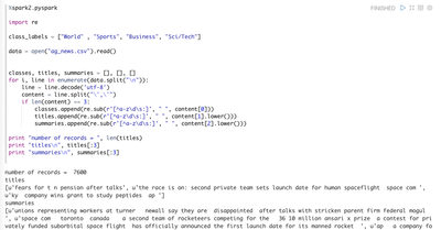
We will use news feed data that has been classified as either 1 (Business), 2 (Sports), 3 (Business) or 4 (Sci/Tech). The data is structured as CSV with fields: class, title, summary. (Note that later processing converts the labels to 0,1,2,3 respectively).

Engineer the data

The class, title and summary fields are appended to their own arrays. Data cleansing is done in the form of punctuation removal and conversion to lowercase.

Convert the data

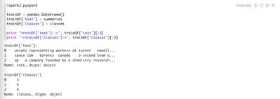
The scikit-learn packages need these arrays to be represented as dataframes, which assign an int to each row of the array inside the data structure.
Note: This first model will use summaries to classify test, as shown in the code.

Vectorize the data

Now we start using the machine learning packages. Here we convert the dataframes into a vector. The vector is a wide n x m matrix with n records and for each record m fields that hold a position for each word detected among all records, and the word frequency for that record and position. This is a sparse matrix since most m positions are not filled. We see from the output that there are 7600 records and 20027 words. The vector shown in the output is partial, showing part of the 0th record with word index positions 11624, 6794, 6996 etc.

Fit (train) the model and determine its accuracy

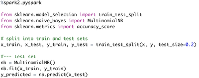
Let’s fit the model. Note that we split the data into a training set with 80% of the records and validation step with the remaining.

Wow! 87% of our tests accurately predicted the text classification. That’s good.

Deeper dive on results

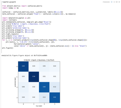
We can look more deeply than the single accuracy score reported above. One way is to generate a confusion matrix as shown below. The confusion matrix shows for any single true single class, the proportion of predictions it made against all predicted classes.

We see that Sports text almost always predicted its classification correctly (0.96). Business and Sci/Tech were a bit more blurred: When Business text was incorrectly predicted, it was usually against Sci/Tech and the converse for Sci/Tech. This all makes sense since Sports vocabulary is quite distinctive and Sci/Tech is often in the Business news.

There are other views of model outcomes ... check the sklearn.metrics api.

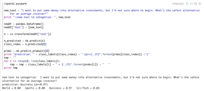
Test the model with a single news feed summary

Now take a single news feed summary and see what the model predicts.

I have run may through the model and it performs quite well. The new text in shown above gets a clear Business classification. When I run news summaries on cultural items (no category in the model), the predictions are low and spread across all categories, as expected.

B. Explore the data

Word and anagram counts

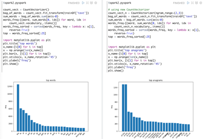
Let’s get the top 25 words and anagrams (phrases, in our case two words) among all training set text that were used to build the model. These are shown below.

Hmm ... there are a lot of common meaningless words involved. Most of these are known as stopwords in natural language processing. Let’s remove the stop words and see if the model improves.

Remove stopwords: retrieve list from file and fill array

The above are stopwords from a file. The below allows you to iteratively add stopwords to the list as you explore the data.

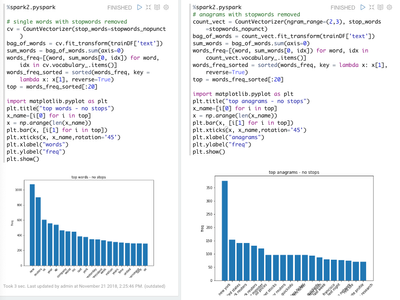
Word and anagram counts with stopwords removed

Now we can see the top 25 words and anagrams after the stopwords are removed. Note how easy this is to do: we instantiate the CountVectorizer exactly as before, but by passing a reference to the stopword list.

This is a good example of how powerful the skilearn libraries are: you interact with the high level apis and the dirty work is done under the surface.

C. Try to improve the model

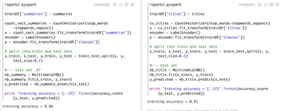
Now we train the same model for news feed summaries with no stop words (left) and for titles and no stopwords.

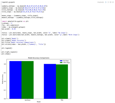
Interesting ... the model using summaries with no stop words is equally accurate as the one with them included in the text. Secondly, the titles model is less accurate than the summary model, but not by much (not bad for classifying text from samples of only 10-20 words).

D. Comparison of model accuracies

I trained each of the below models 5 times each: news feed text from summaries (no stops, with stops) and from titles (no stops, with stops). I averaged the accuracies and plotted as shown below.

E. Conclusions

Main Conclusions are:

Naive Bayes effectively classified text particularly given small text sizes (news titles, news summaries of 1-4 sentences)
Summaries classified with more accuracy than titles, but not by much considering how few attributes (words) are in a single title
Removing stop words had no significant effect on model accuracy. This should not be surprising because stop words are expected to be represented equally among classifications
Recommended model: summary with stop words retained, because it has highest accuracy and lower complexity of code and lower processing needs than the equally accurate summary with stop words removed model
This model is susceptible to overfitting because the stories represent a window of time and its text (news words) accordingly is biased toward the “current” events at that time.