Community Articles
- Cloudera Community
- Support
- Community Articles
- Tuning Hyperparameters with Experiments feature on...
- Subscribe to RSS Feed
- Mark as New
- Mark as Read
- Bookmark
- Subscribe
- Printer Friendly Page
- Report Inappropriate Content
- Subscribe to RSS Feed
- Mark as New
- Mark as Read
- Bookmark
- Subscribe
- Printer Friendly Page
- Report Inappropriate Content
Created on
04-20-2023
09:00 AM
- edited on
04-21-2026
12:16 AM
by
GrazittiAPI
Introduction
Data Scientists work iteratively in a stochastic space to build models for addressing business use cases. In a typical Machine Learning workflow, Data Scientists iterate by combining their training data with an array of algorithms. In this activity, called model training and evaluation, there are two decisions being made. The first decision involves identifying the dataset for training and testing. Identifying a dataset that is representative of the actual data that the ML system is likely to encounter in a real-life scenario is a key success factor for the system. This helps a trained model to make better predictions when applied to real data. The second decision involves comparing different algorithms around a set of performance metrics. Since both of these decisions tend to be more heuristic-based rather than rule-based, this process is also called experimentation in machine learning parlance.
Cloudera AI has simplified experimentation during the model training step of a Data Science workflow with the integration of MLflow Tracking. This managed MLflow component, together with Model Registry and Feature Store (planned for future CML releases) will greatly aid in improving the productivity of data science teams in scaling their training workflows and deploying their models. Here is a quick look at what MLflow Experiment Tracking looks like in CML. Later we will learn how to analyze experiment runs in detail.
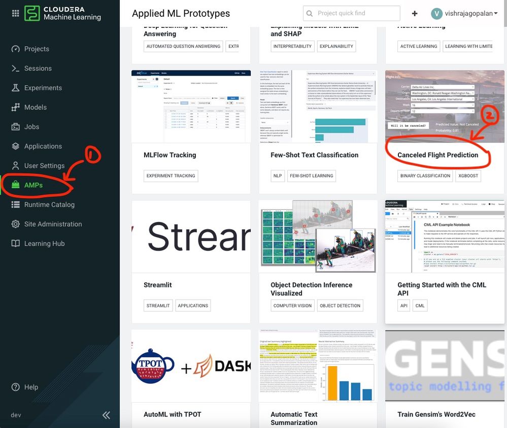
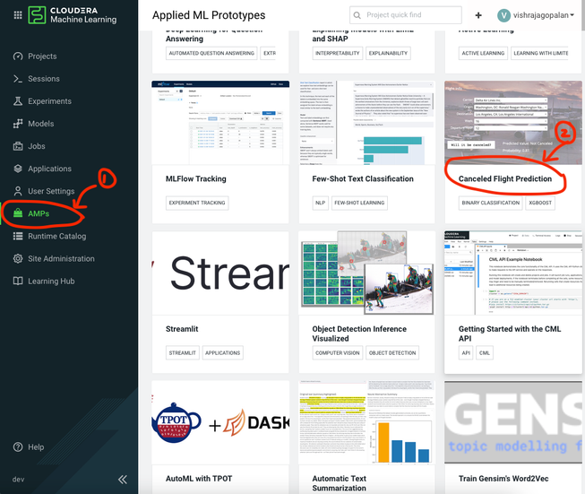
This article demonstrates how to get started with the new and improved experiments, powered by MLFlow, in Cloudera Machine Learning using a use case of flight cancellation prediction. This use case is available as an Applied Machine Learning Prototype (AMP) on the CML platform. For new users of the Cloudera Machine Learning platform, AMPs provide end-to-end example machine learning projects in CML (refer to image below). To know more about AMPs you can check the documentation here.
AMPs provide end-to-end example machine learning projects in CML (refer to the image below). To know more about AMPs you can check the documentation here.
Pre-requisites
Access to a Cloudera Machine Learning environment
A CML Workspace with a minimum compute resources of 16 vCPU / 32 GB RAM
Credits and Resources for further reading
Hyperopt: http://hyperopt.github.io/hyperopt/
XGboost: https://xgboost.readthedocs.io/en/stable/
Getting Started with CML Experiments Feature
Setup up the CML Project :
Note: Optional. Skip this section if you know how to launch a CML AMP by directly selecting the Flight Cancellation Prediction AMP
This section provides a step-by-step explanation of how to set up a CML project that will be subsequently used for demonstrating the Experiments feature in the next section. If you are familiar with setting up a project using a Cloudera Machine Learning AMP, you can directly launch the CML AMP for Flight Cancellation Prediction from the AMPs menu item and skip this section.
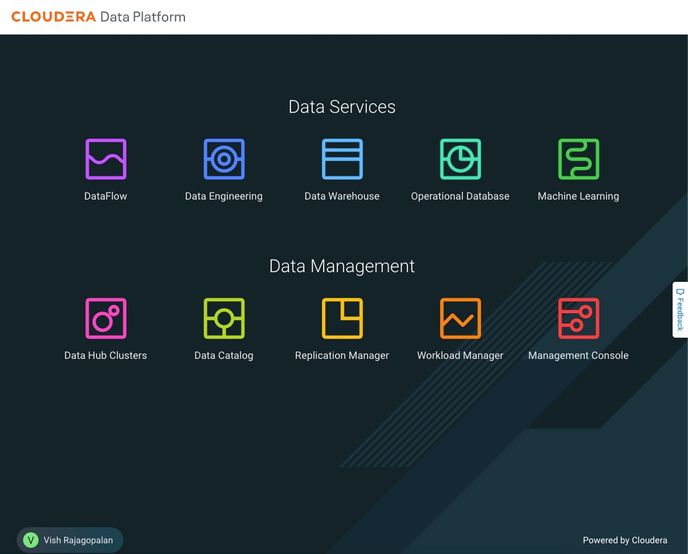
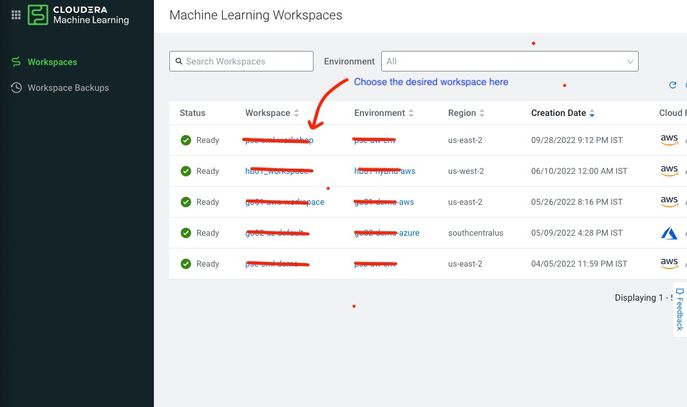
Let us now start From the Control Pane click on Machine Learning and choose a workspace where you want to create a project ( refer to the images below)
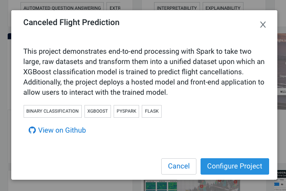
To start using the Experiments feature in CML, let us first set up a CML Project. As mentioned earlier, a convenient way to quickstart use cases in CML is the AMPs and we will use one such AMP to work with the MLflow Experiments feature. There are more than one ways to create AMPs within the CML platform. We will use the intuitive option of creating the AMP by choosing the AMP menu item and selecting the cancellation prediction AMP. On the subsequent pop-up, click on Configure Project.
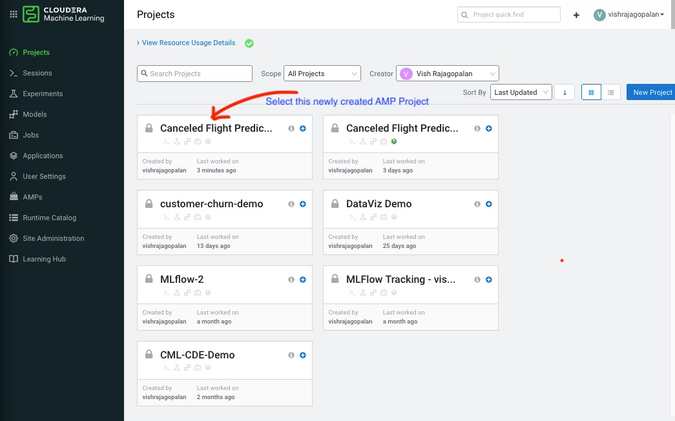
Next, you need to go back to your Projects and select the newly created Project called Canceled Flight Predictions ( see below)
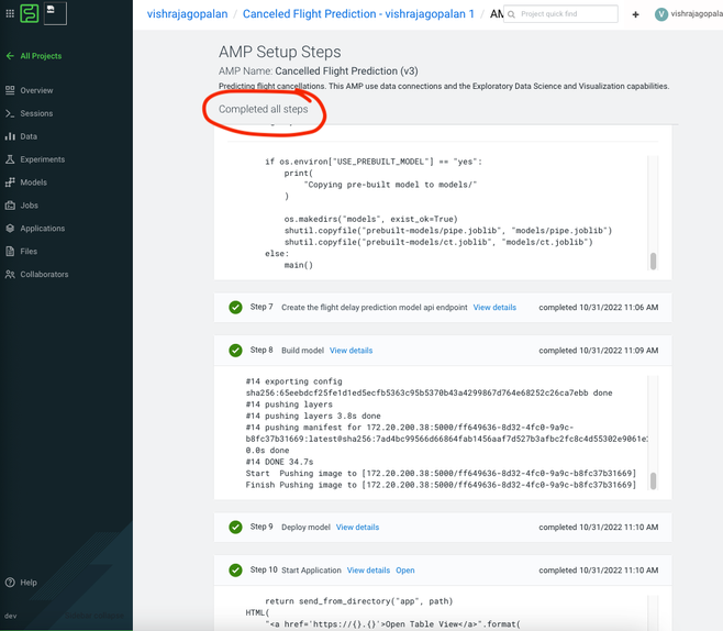
As a final step to project creation, you need to now click Launch Project, which builds the project files as well as creates project artifacts. Use the default Engine and Runtime parameters and launch the project. This Kicks off the AMP setup Steps as below and you should wait for all the 10 Steps to be completed to ensure that the project has been installed in your workspace ( Refer to figure below).
“Just Enough” MLflow Library Explanation
This section provides some basic information on MLflow experiments. You are encouraged to use this as a starting point and then dive deeper into official documentation on your own.
- Set up an Experiment: When you are starting to train model Hyperparameters, use a new experiment name as a best practice with a call to mlflow.set_experiment (“uniqueName”) function. If you do not use this function, a default experiment is created for you. However, this may lead to headaches later when trying to track results, so best to pick a name.
- Runs of an Experiment: Each combination of parameter values that one would like to change in an experiment is tracked as a Run. At the end of an Experiment, you are comparing the outcomes across multiple runs. To start a new run, call the function mlflow.start_run() function
- Tracking the metric: This function tracks the metric of interest with a call to function mlflow.track_metric(). In the example stated above it could be any or all of the parameters described ( e.g. learning rate, or Optimizer type). Finally, you also need to track the outcome metric (e.g. accuracy or error). The way to track the outcome metrics is also to call the function mlflow.track_metric().
Launching Experiments in CML.
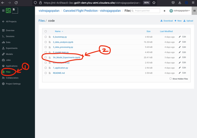
Download the Ipython notebook t called 5A_Model_Experiments.ipynb from the GitHub repo here. This is the Ipython notebook that you will use for the Hyperparameter search using the Experiments feature in CML. Upload this Jupyter notebook into the code folder. You should now be able to see the uploaded file below. If you are not sure how to upload, just click the Files section, navigate to the code folder, and click the upload option seen in the top right corner.
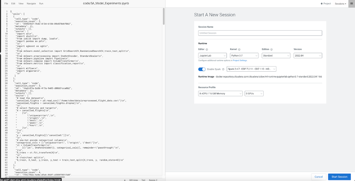
Next, click on Open in “Workbench” and select Start a new Session. Here choose at least the resource Profile below or higher as shown below:
The Python notebook provides a step-by-step explanation of the different steps in MLflow Experiments creation. I recommend a code walkthrough and reading the code comments and documentation to understand the steps performed.
Here is a summary of all the key steps in this notebook:
- Setup of necessary packages such as scikitlearn, mlflow, and XGBoost for model development
- Ingestion of preprocessed data: Here we are ingesting a preprocessed file created by the AMP
- Installing Hyperopt - We will use this open-source library for “smart hyperparameter search”
- Hyperparameter search space and search strategy
- Comparison of model performance between baseline and the best Hyperparameters
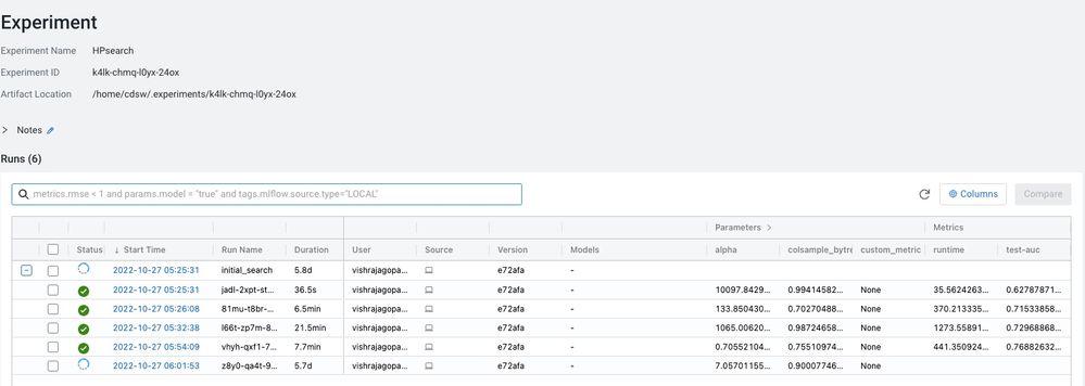
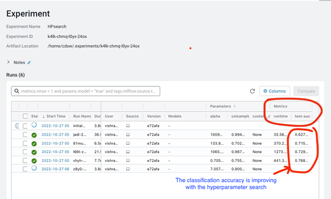
Go ahead and execute all the steps by clicking “Run All” for the Notebook from the Run menu. This executes all of the above steps and, in approximately 10-15 minutes, the first set of Experiment runs will be logged. Next, come back to the Project work area and click on the Experiments menu. You should see the experiment name “HPsearch” below:
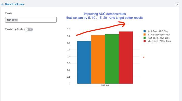
Click on the “HP Search” above to bring the Experiment Details Page below ( Figure XX: Image - ExperimentDetails.jpeg). This shows the Information captured by MLflow tracking. The Metrics column is of interest to us because we are interested in tracking the accuracy of our flight prediction model, as measured by metrics “test-auc” (Area Under Curve). We can observe that the test-auc values are increasing, which means that our search for Hyperparameters is going to lead to improvement in the model. The higher our test-auc value the more likely our flight cancellation prediction service is likely to predict accurately in real-world scenarios.
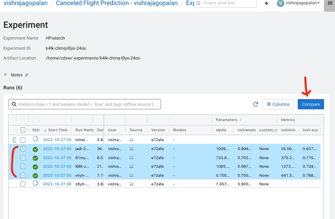
One of the nicest features of MLflow tracking is the multiple options available for us to compare our experiment runs. As a next step, select the checkboxes against the completed runs and then click on the compare button. This allows us to compare the Runs in tabular and graphical formats, as shown below. Please note, you may need to change the timeout to increase the number of runs in the code below:
# This will take a considerable time and computing power to tune. For the purpose of efficiency, we are stopping the run at 10 minutes
with mlflow.start_run(run_name='xgb_loss_threshold'):
best_params = fmin(
fn=train_model,
space=search_space,
algo=tpe.suggest,
loss_threshold=-0.7, # stop the grid search once we've reached an AUC of 0.92 or higher
timeout=60*10 # stop after 10 minutes regardless if we reach an AUC of 0.92
)
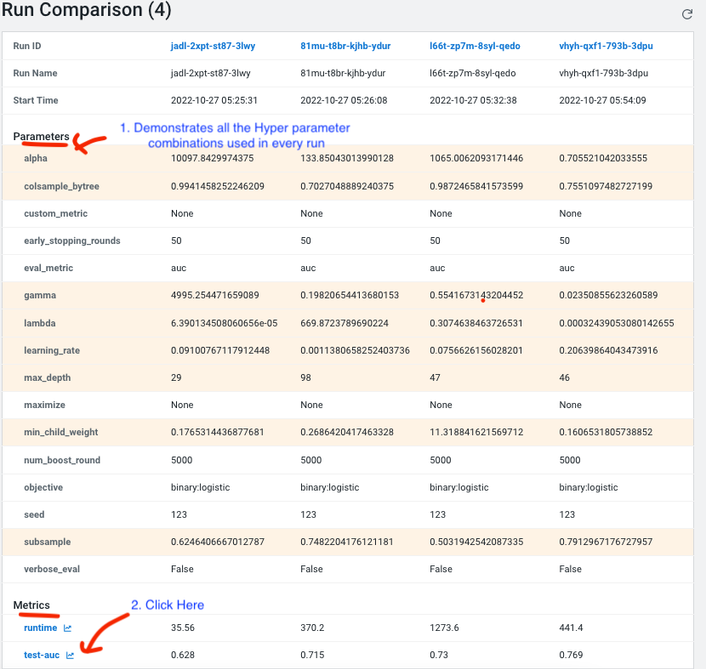
The “Run Comparison” page demonstrates the Hyperparameters for every experiment run and the outcomes from that run in the Parameters and Metrics section as shown in the images below. Notice that you can now see improvements in accuracy metric graphically by just clicking on “test-auc”.
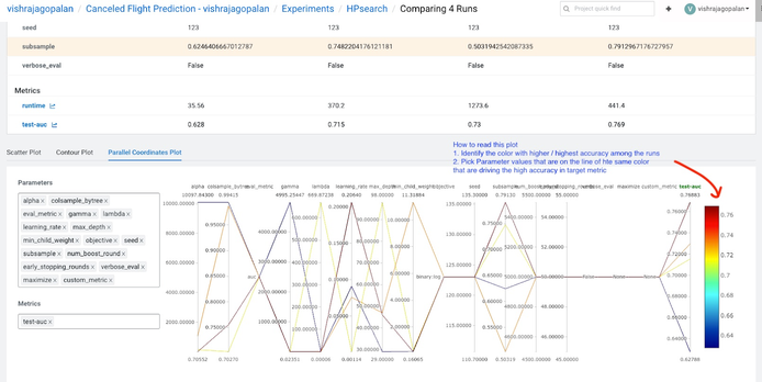
Finally, what should we do, if we would like to handpick the Hyperparameters combinations across different runs? We can do this by going back to the comparisons page (follow the same approach described earlier of selecting the runs and clicking on the compare button). Now, scroll down to the choice of graphs provided by MLflow. There are multiple choices here, but the Parallel Coordinates Plot provides a great way for you to hand pick Hyperparameters that influence the best outcomes ( refer to Figure XX - Image: ParalleCoordinatesPlot.jpeg). The chart explains the best way to pick the best hyperparameters among runs compared.
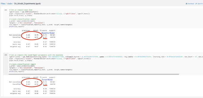
Until now, we have used the Experiments feature to compare the different runs. Finally, let us make a comparison between our baseline model and a model built with optimal Hyperparameters obtained from our experiments. We need to check if it is worthwhile training our model with these chosen parameters.
If we go back to the 5A_Experiments.ipynb notebook and compare the outcomes of the baseline model and the tuned model, we can notice that there is an increase in the accuracy of cancellation predictions that we have achieved through Hyperparameter tuning.
Summary:
This article demonstrates how the Experiments feature in Cloudera Machine Learning can be used for empirical experimentation in Machine Learning workflows. We have taken a typical Data
Science workflow uses the case of tuning the Hyperparameters of a prediction model to show how this can be achieved and the different options available to us in the Experiments feature to track our experiments and compare the outcomes of the experiment runs for improved model outcomes. The MLflow package is available as a part of the Cloudera Machine Learning experience (no pip install needed) and by using a set of API calls, we are able to quickly set up experiments in our ML projects. This feature, using managed MLflow tracking, eases the life of the Data Science team during the critical training phase of model development and results in improved productivity through accurate and easy logging of training runs on ML models.
